For importing CSV data into a PostgreSQL database one can use the COPY command as follows:

COPY AISInput(T, TypeOfMobile, MMSI, Latitude, Longitude, NavigationalStatus,
  ROT, SOG, COG, Heading, IMO, CallSign, Name, ShipType, CargoType, Width, Length,
  TypeOfPositionFixingDevice, Draught, Destination, ETA, DataSourceType,
  SizeA, SizeB, SizeC, SizeD)
FROM '/home/mobilitydb/DanishAIS/aisdk_20180401.csv' DELIMITER  ',' CSV HEADER;
				

This import took about 3 minutes on my machine, which is an average laptop. The CSV file has 10,619,212 rows, all of which were correctly imported. For bigger datasets, one could alternative could use the program pgloader.

We clean up some of the fields in the table and create spatial points with the following command.

UPDATE AISInput SET
  NavigationalStatus = CASE NavigationalStatus WHEN 'Unknown value' THEN NULL END,
  IMO = CASE IMO WHEN 'Unknown' THEN NULL END,
  ShipType = CASE ShipType WHEN 'Undefined' THEN NULL END,
  TypeOfPositionFixingDevice = CASE TypeOfPositionFixingDevice
  WHEN 'Undefined' THEN NULL END,
  Geom = ST_SetSRID( ST_MakePoint( Longitude, Latitude ), 4326);
				

This took about 5 minutes on my machine. Let's visualize the spatial points on QGIS.

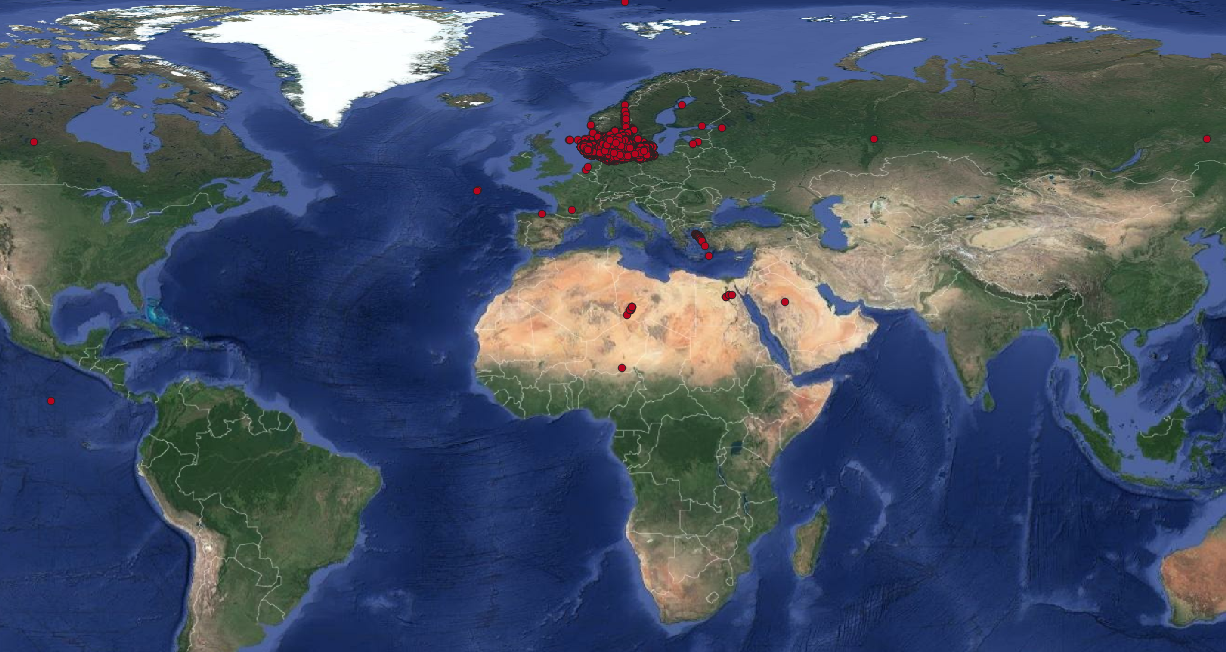
Clearly, there are noise points that are far away from Denmark or even outside earth. This module will not discuss a thorough data cleaning. However, we do some basic cleaning in order to be able to construct trajectories:

CREATE TABLE AISInputFiltered AS
SELECT DISTINCT ON(MMSI,T) *
FROM AISInput
WHERE Longitude BETWEEN -16.1 and 32.88 AND Latitude BETWEEN 40.18 AND 84.17;
-- Query returned successfully: 10357703 rows affected, 01:14 minutes execution time.
SELECT COUNT(*) FROM AISInputFiltered;
--10357703