We will start by looking at a single airplane. Grafana proves to be a good way to quickly visualize our dataset and can be useful to support pre-processing and cleaning. If using a connection to the Azure database, required tables are already created.
A full description of each parameter is included in the OpenSky original dataset readme. The table structure in the Azure dataset after loading and transformations looks like the following:
Figure 3.1. First row of table “single_airframe”, with 24hrs of flight information for airplane “c827a6”
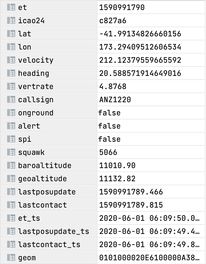 |
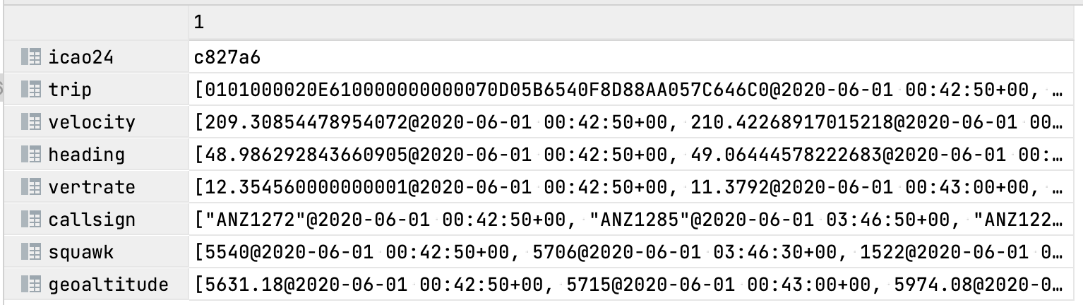
Figure 3.2. Full table “single_airframe_traj” for airplane “c827a6” with data in mobilityDB trajectories format
 |
Make Sure you are visualizing the data in the correct timezone. The data we had was in UTC. To change the timezone,
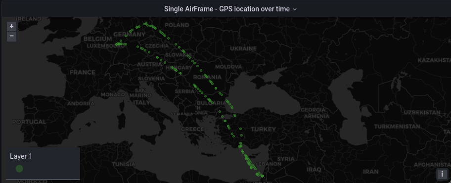
Let’s visualize the latitude and longitude coordinates of an airplane’s journey throughout the day. For this one we will not color the geo-markers, but it is possible to color them using some criterion.
-
Add a new panel
-
Select “OpenSkyLOCAL” as the data source
-
In Format as, change “Time series” to “Table” and choose “Edit SQL”
-
Here you can add your SQL queries. Let’s replace the existing query with the following SQL script:
-- icao24 is the unique identifier for each airframe (airplane) SELECT et_ts, icao24, lat, lon -- TABLESAMPLE SYSTEM (n) returns only n% of the data from the table. FROM flights TABLESAMPLE SYSTEM (5) WHERE icao24 IN ('738286') AND $__timeFilter(et_ts) -
Change the visualization type to “Geomap”.
-
The options (visualization settings - on the right side of the screen) should be as follows:
Panel Options
-
Title →GPS location over time
Map View
-
Initial view: For this one zoom in on the visualization on the panel as you see fit and then click “use current map settings ” button.
Data Layer
-
Layer type: → “markers”
-
Style size → Fixed Value: 2
-
Color → Green
-
In this visualization we can see that the airplane is visiting different countries and almost completing a loop. This indicates that there are more than 1 trips (flights) completed by this single airplane. The coordinates are sparse because we are sampling the results using “TABLESAMPLE SYSTEM (5)” in our query. This is done to speed up the visualization.
Following the similar steps to add a Geomap panel as before, we include the following SQL script. Note $__timeFilter() is a Grafana global variable. This global variable will inject time constraint SQL-conditions from Grafana’s time range panel.
-
In Format as, use “Time series”
SELECT
  et_ts AS "time",
  velocity
FROM flights
WHERE icao24 = 'c827a6' AND $__timeFilter(et_ts)
-
Change the visualization type to “Time Series”.
-
The options (visualization settings - on the right side of the screen) should be as follows:
Panel Options
-
Title → Single AirFrame - Velocity vs Time
-
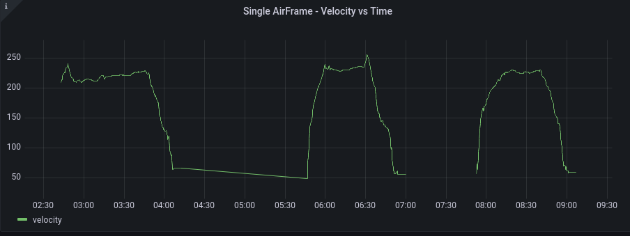
In the visualization we can see clearly that on this day, this airframe took 3 flights. That is why its speed curve has 3 humps. The zero speed towards the end of each hump is a clear indicator that plane stopped, thus it must have completed its flight.
Follow the similar steps to add a Geomap panel as before, we include the following SQL script.
-
In Format as, we have “Time series”
SELECT
  et_ts AS "time",
  baroaltitude, geoaltitude
FROM flights
WHERE icao24 = 'c827a6' AND $__timeFilter(et_ts)
-
Change the visualization type to “Time Series”.
-
The options (visualization settings - on the right side of the screen) should be as follows:
Panel Options
-
Title → Single AirFrame - Altitude vs Time
-
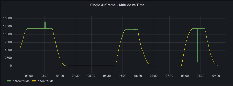
In the visualization we can again see that on this day, the airframe took 3 flights, as altitude reaches zero between each flight. There is some noise in the data, which appear as spikes. This would be almost impossible to spot in a tabular format, but on a line graph these data anomalies can be easily identified.
Follow the similar steps to add a Geomap panel as before, we include the following SQL script.
-
In Format as, we have “Time series”
SELECT
  et_ts AS "time",
  vertrate
FROM flights
WHERE icao24 = 'c827a6' AND $__timeFilter(et_ts)
-
Change the visualization type to “Time Series”.
-
The options (visualization settings - on the right side of the screen) should be as follows:
Panel Options
-
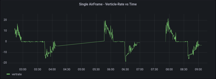
Title → Single AirFrame - Verticle-Rate vs Time
-
The positive values here represents the ascent of the plane. While at cruising altitude, the plane has almost zero vertical-rate and during decent this value becomes negative. So a sequence of positive values, then zero values followed by negative values would represent a single flight.
The callsign is a unique identifier used for a specific flight path. For example, ANZ1220 is the callsign of the Air New Zealand flight 1220 from Queenstown to Auckland in New Zealand. It is possible for single airplane to make the same flight more than once in a 24hr period if it goes back and forth. This information will be used in later queries to partition an airplanes data into multiple flights.
We can find the time at which the callsign of an airplane changes with the following steps.
-
In Format as, we have “Table”
SELECT
  min(et_ts) AS "time", callsign
FROM flights
WHERE icao24 = 'c827a6'
GROUP BY callsign
-
Change the visualization type to “Table”.
-
The options (visualization settings - on the right side of the screen) should be as follows:
Panel Options
-
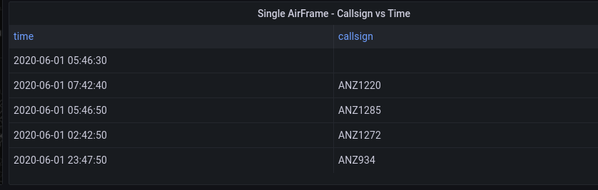
Title → Single AirFrame - Callsign vs Time
-
In the visualization we can see that this airplane completed 3 flights and started the 4th one towards the very end of the day. We also see there is some NULL data in the callsign column which is why the first timestamp doesn’t have a corresponding callsign.