For the following queries, we will make use of trajectories for aggregation and creating effective splits in our data based on parameters that change in time.
This step is completed once, only on the ingestion of data. It is shown below to provide an understanding of how to do it. With temporal datatypes and mobilityDB functionality, we can see the queries are very intuitive to create.
We first create a geometry point. This treats each latitude and longitude as a point in space. 4326 is the SRID.
ALTER TABLE flights
    ADD COLUMN geom geometry(Point, 4326);

UPDATE flights SET
  geom = ST_SetSRID( ST_MakePoint( lon, lat ), 4326);
Now we are ready to construct airframe or airplane trajectories out of their individual observations. Each “icao24” in our dataset represents a single airplane.
We can create a composite index on icao24 (unique to each plane) and et_ts (timestamps of observations) to help improve the performance of trajectory generation.
CREATE INDEX icao24_time_index
    ON flights (icao24, et_ts);
We create trajectories for a single airframe because:
-
this query serves as a simple example of how to use mobilityDB to create trajectories
-
these kind of trajectories can be very important for plane manufacturer, as they are interested in the airplane’s analysis.
-
we are creating the building blocks for future queries. Each row would represent a single flight, where flight is identified by icao24 & callsign.
CREATE TABLE airframe_traj(icao24, trip, velocity, heading, vertrate, callsign, squawk,
                           geoaltitude) AS
SELECT icao24,
       tgeompoint_seq(array_agg(tgeompoint_inst(geom, et_ts) ORDER BY et_ts)
                      FILTER (WHERE geom IS NOT NULL)),
       tfloat_seq(array_agg(tfloat_inst(velocity, et_ts) ORDER BY et_ts)
                  FILTER (WHERE velocity IS NOT NULL)),
       tfloat_seq(array_agg(tfloat_inst(heading, et_ts) ORDER BY et_ts)
                  FILTER (WHERE heading IS NOT NULL)),
       tfloat_seq(array_agg(tfloat_inst(vertrate, et_ts) ORDER BY et_ts)
                  FILTER (WHERE vertrate IS NOT NULL)),
       ttext_seq(array_agg(ttext_inst(callsign, et_ts) ORDER BY et_ts)
                 FILTER (WHERE callsign IS NOT NULL)),
       tint_seq(array_agg(tint_inst(squawk, et_ts) ORDER BY et_ts)
                FILTER (WHERE squawk IS NOT NULL)),
       tfloat_seq(array_agg(tfloat_inst(geoaltitude, et_ts) ORDER BY et_ts)
                  FILTER (WHERE geoaltitude IS NOT NULL))
FROM flights
GROUP BY icao24;
Here we create a new table for all the trajectories. We select all the attributes of interest that change over time. We can follow the transformation from the inner call to the outer call:
-
tgeompoint_inst: combines each geometry point(lat, long) with the timestamp where that point existed
-
array_agg: aggregates all the instants together into a single array for each item in the group by. In this case, it will create an array for each icao24
-
tgeompoint_seq: constructs the array as a sequence which can be manipulated with mobilityDB functionality. The same approach is used for each trajectory, with the function used changing depending on the datatype.
Right now we have, in a single row, an airframe’s (where an airframe is a single physical airplane) entire day’s trip information. We would like to segment that information per flight (an airframe flying under a specific callsign). This query segments the airframe trajectories (in temporal columns) based on the time period of the callsign. Below we explain the query and the reason behind segmenting the data this way.
-- Each row from airframe will create a new row in flight_traj depending on when the
-- callsign changes, regardless of whether a plane repeats the same flight multiple
-- times in any period

-- Airplane123 (airframe_traj) |-------------------------|
-- Flightpath1 (flight_traj)   |-----|
-- Flightpath2 (flight_traj)         |--------|
-- Flightpath1 (flight_traj)                  |-------|
-- Flightpath3 (flight_traj)                          |--|
CREATE TABLE flight_traj(icao24, callsign, flight_period, trip, velocity, heading,
                         vertrate, squawk, geoaltitude)
AS
    -- callsign sequence unpacked into rows to split all other temporal sequences.
WITH airframe_traj_with_unpacked_callsign AS
         (SELECT icao24,
                 trip,
                 velocity,
                 heading,
                 vertrate,
                 squawk,
                 geoaltitude,
                 startValue(unnest(segments(callsign))) AS start_value_callsign,
                 unnest(segments(callsign))::period     AS callsign_segment_period
          FROM airframe_traj)

SELECT icao24                                         AS icao24,
       start_value_callsign                           AS callsign,
       callsign_segment_period                        AS flight_period,
       atPeriod(trip, callsign_segment_period)        AS trip,
       atPeriod(velocity, callsign_segment_period)    AS velocity,
       atPeriod(heading, callsign_segment_period)     AS heading,
       atPeriod(vertrate, callsign_segment_period)    AS vertrate,
       atPeriod(squawk, callsign_segment_period)      AS squawk,
       atPeriod(geoaltitude, callsign_segment_period) AS geoaltitude
FROM airframe_traj_with_unpacked_callsign;
Note:
We could have tried to
create the above (table ”flight_traj”) per flight trajectories
by simply including “callsign” in the GROUP BY
statement in the query used to create the previous
airframe_traj table
(GROUP BY icao24, callsign;).
The problem with this solution: This approach would put the trajectory data of 2 distinct flights where that airplane and flight number are the same in a single row, which is not correct.
MobilityDB functions helped us avoid the use of several hardcoded conditions that depend on user knowledge of the data. This approach is very generic and can be applied anytime we want to split a trajectory by the inflection points in time of some other trajectory.
We can now use our trajectories to pull flight specific statistics very easily.
-
In Format as, we have “Table”
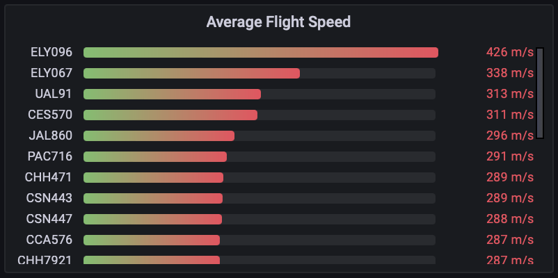
-- Average flight speeds during flight SELECT callsign,twavg(velocity) AS average_velocity FROM flight_traj WHERE twavg(velocity)IS NOT NULL -- drop rows without velocity data AND twavg(velocity) < 1500 -- removes erroneous data ORDER BY twavg(velocity) desc; -
Change the visualization type to “Bar gauge”.
-
The options (visualization settings - on the right side of the screen) should be as follows
Panel Options
-
Title → Average Flight Speed
Bar gauge
-
Orientation → Horizontal
Standard Options
-
Unit → meters/second (m/s)
-
Min → 200
The settings we adjust improve the visualization by cutting the bar graph values of 0-200, improving the resolution at higher ranges to see differences.
-
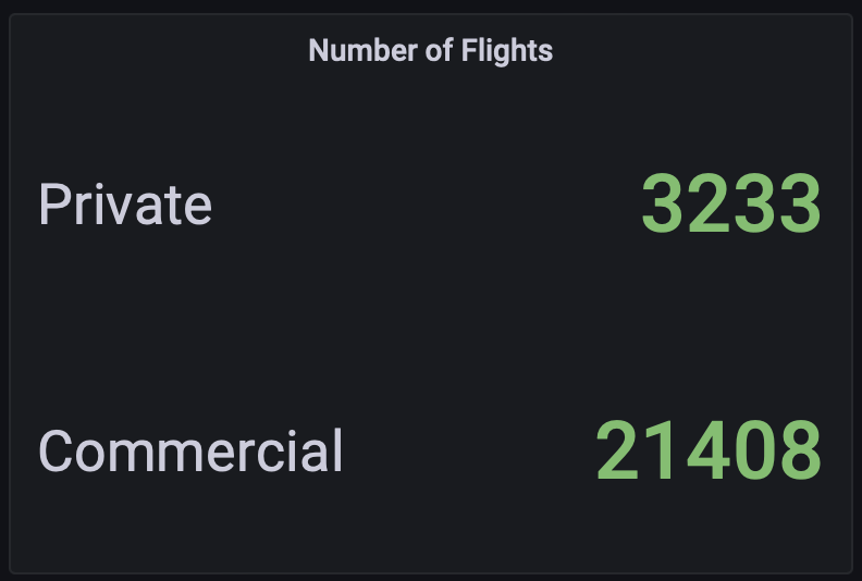
We can easily combine results from multiple queries in the same visualization in Grafana, simplifying the queries themselves. Here we apply some domain knowledge of sport pilot aircraft license limits for altitude and speed to provide an estimated count of each.
-
In Format as, we have “Table”
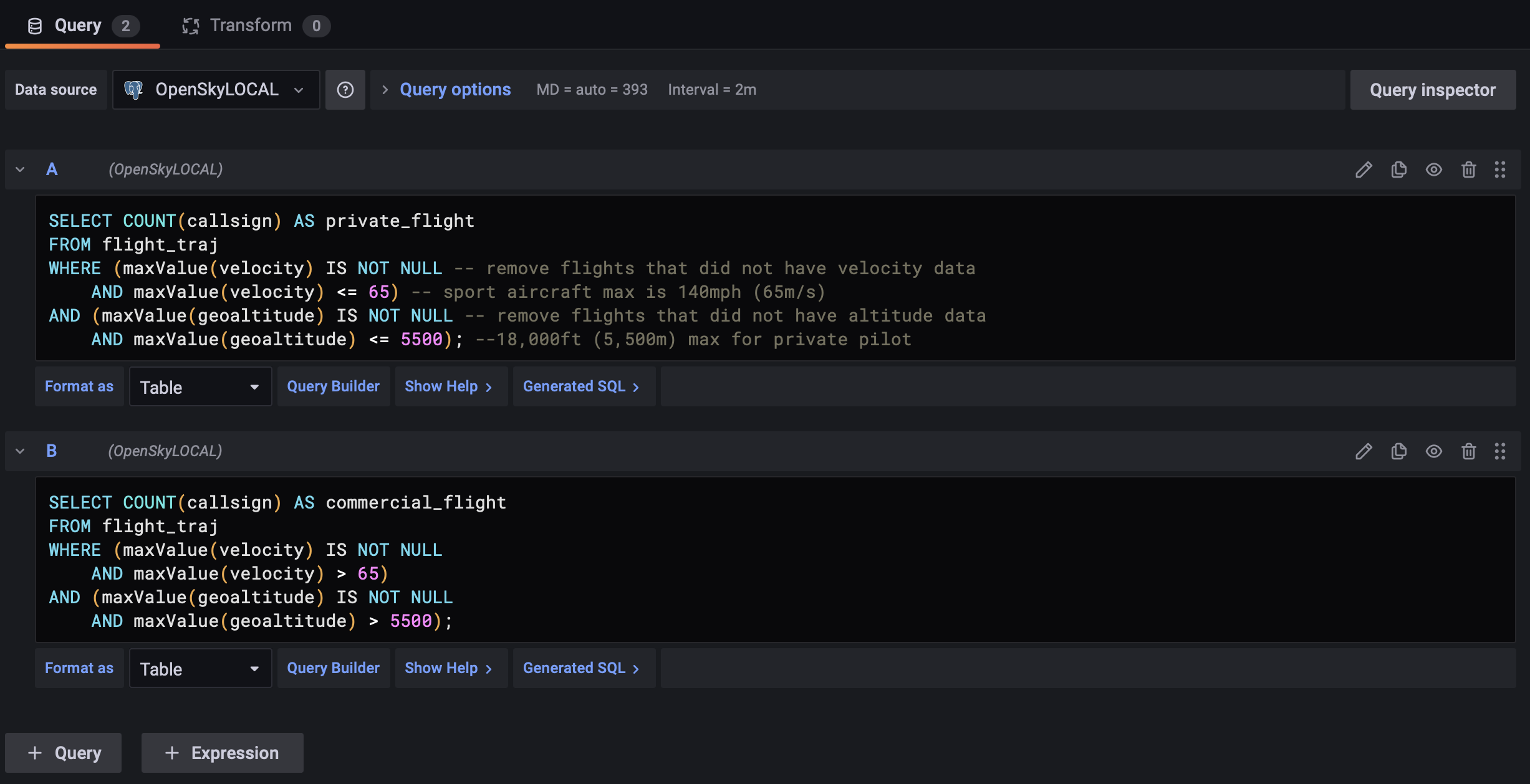
-- Flights completed by private pilots (estimate)
SELECT COUNT(callsign) AS private_flight
FROM flight_traj
WHERE (maxValue(velocity) IS NOT NULL -- remove flights without velocity
    AND maxValue(velocity) <= 65) -- sport aircraft max is 140mph (65m/s)
AND (maxValue(geoaltitude) IS NOT NULL -- remove flights without altitude
    AND maxValue(geoaltitude) <= 5500); --18,000ft (5,500m) max for private pilot

-- Count of commercial flights (estimate)
SELECT COUNT(callsign) AS commercial_flight
FROM flight_traj
WHERE (maxValue(velocity) IS NOT NULL
    AND maxValue(velocity) > 65)
AND (maxValue(geoaltitude) IS NOT NULL
    AND maxValue(geoaltitude) > 5500);
In Grafana, when we are in the query editor we can click on “+ Query” at the bottom to add multiple queries that provide different results.
-
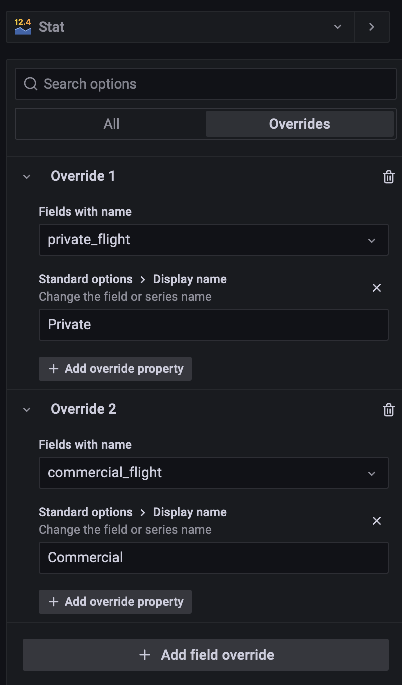
Change the visualization type to “Stat”.
To label the data for each result separately, choose “Overrides” at the top of the options panel on the right. Here you can override global panel settings for specific attributes as shown below.
The final statistics visualization will look like this:
Note: This query makes used of a sample set of data that has 200 flights to return results. “flight_traj_sample” is just a sampled version of “flight_traj”. As of the writing of this workshop, Grafana does not support display of vectors, and so individual latitude and longitude points are used as a proxy.
In order to make the query use Grafana global time range panel replace the hard-coded timestamps with the ‘[${__from:date}, ${__to:date} )’.
WITH
-- The flight_traj_time_slice CTE is clipping all the temporal columns
-- to the user specified time-range.
flight_traj_time_slice (icao24, callsign, time_slice_trip, time_slice_geoaltitude,
                        time_slice_vertrate) AS
    (SELECT icao24,
            callsign,
            atPeriod(trip, period '[2020-06-01 03:00:00, 2020-06-01 20:30:00)'),
            atPeriod(geoaltitude, period '[2020-06-01 03:00:00, 2020-06-01 20:30:00)'),
            atPeriod(vertrate,
                     period '[2020-06-01 03:00:00, 2020-06-01 20:30:00)')
     FROM flight_traj_sample TABLESAMPLE SYSTEM (20)),

-- There are 3 things happening in the flight_traj_time_slice_ascent CTE:
-- 1. atRange: Clips the temporal data to create ranges where the vertrate
--  was between '[1, 20]'. This vertrate means an aircraft was ascending.
-- 2. sequenceN: Selects the first sequence from the generated sequences.
--  This first sequence is takeoff and eliminates mid-flight ascents.
-- 3. atPeriod: Returns the period of the first sequence.
flight_traj_time_slice_ascent(icao24, callsign, ascending_trip, ascending_geoaltitude,
                              ascending_vertrate) AS
    (SELECT icao24,
            callsign,
            atPeriod(time_slice_trip,
                     period(sequenceN(
                         atRange(time_slice_vertrate, floatrange '[1,20]'), 1))),
            atPeriod(time_slice_geoaltitude,
                     period(sequenceN(atRange(time_slice_vertrate, floatrange '[1,20]'),
                                      1))),
            atPeriod(time_slice_vertrate,
                     period(sequenceN(atRange(time_slice_vertrate, floatrange '[1,20]'),
                                      1)))
     FROM flight_traj_time_slice),

-- The final_output CTE uses unnest to unpack the temporal data into rows for
-- visualization in Grafana. Each row will contain a latitude, longitude and the altitude
-- and vertrate at those locations.
final_output AS
    (SELECT icao24,
            callsign,
            getValue(unnest(instants(ascending_geoaltitude))) AS geoaltitude,
            getValue(unnest(instants(ascending_vertrate)))    AS vertrate,
            ST_X(getValue(unnest(instants(ascending_trip))))  AS lon,
            ST_Y(getValue(unnest(instants(ascending_trip))))  AS lat
     FROM flight_traj_time_slice_ascent)

SELECT *
FROM final_output
WHERE vertrate IS NOT NULL
  AND geoaltitude IS NOT NULL;
Tips for QGIS visualization: QGIS uses geometry points for visualization, so for that in the third CTE you can use trajectory function on ascending_trip and unnest the result.
We will modify make the follow adjustments for the visualization.
-
Change the visualization type to “Geomap”.
-
The options (visualization settings - on the right side of the screen) should be as follows:
Panel Options
-
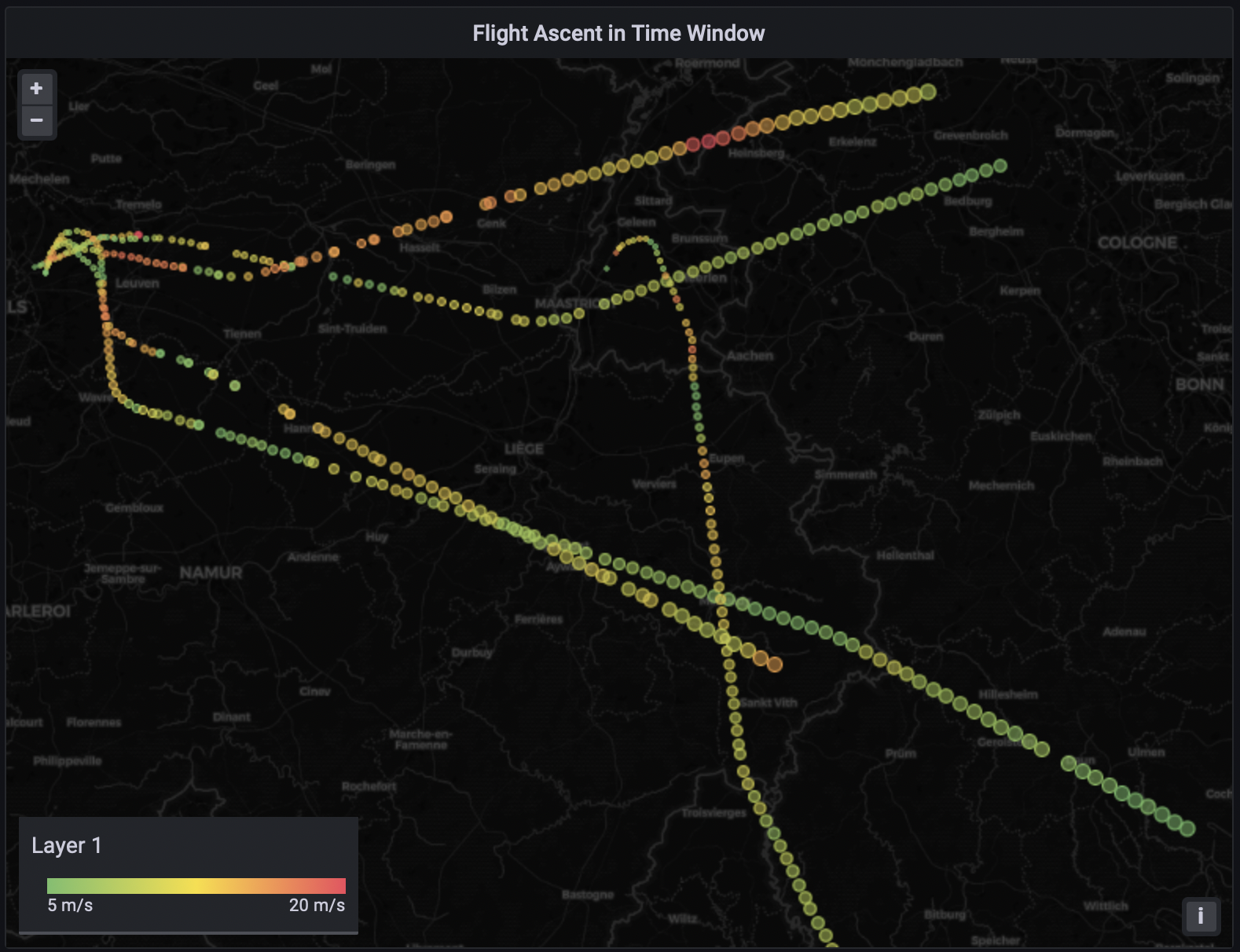
Title → Flight Ascent in Time Window
Data Layer:
-
Layer type: Markers
-
Location: Coords
-
Latitude field: lat
-
Longitude field: lon
-
Styles
-
Size: geoaltitude
-
Min: 1
-
Max: 5
-
Color: vertrate
-
Fill opacity: 0.5
-
Standard Options:
-
Unit: meters/second (m/s)
-
Color scheme: Green-Yellow-Red (by value)
-
-
We will also add a manual override (top right of panel options, beside "All") to limit the minimum value of vertebrate. This will make all values below the minimum the same color, making larger values more obvious. This can be used to quickly pinpoint locations where a large rate of ascent existed.
Overrides
-
Min: 5
-
Max: 20
-
Add field override > Fields with name > vertrate
-
Here is a zoomed in version of how each individual flight ascent will look, as well as a view of multiple flights at the same time. The marker size is increasing with altitude, and the color is showing more aggressive vertical ascent rates. We can see towards the end of the visualized ascent period, there is a short increased vertical ascent rate.
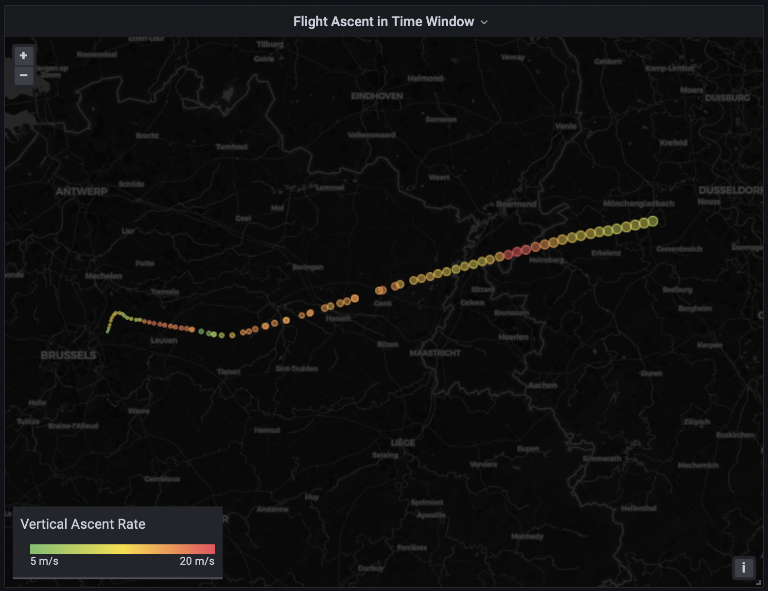
The final visualization will look like the below.