The total distance traveled by all ships:

SELECT SUM( length( Trip ) ) FROM Ships;
--500433519.121321
				

This query uses the length function to compute per trip the sailing distance in meters. We then aggregate over all trips and calculate the sum. Let's have a more detailed look, and generate a histogram of trip lengths:

WITH buckets (bucketNo, RangeKM) AS (
  SELECT 1, floatrange '[0, 0]' UNION
  SELECT 2, floatrange '(0, 50)' UNION
  SELECT 3, floatrange '[50, 100)' UNION
  SELECT 4, floatrange '[100, 200)' UNION
  SELECT 5, floatrange '[200, 500)' UNION
  SELECT 6, floatrange '[500, 1500)' UNION
  SELECT 7, floatrange '[1500, 10000)' ),
histogram AS (
  SELECT bucketNo, RangeKM, count(MMSI) as freq
  FROM buckets left outer join Ships on (length(Trip)/1000) <@ RangeKM
  GROUP BY bucketNo, RangeKM
  ORDER BY bucketNo, RangeKM
)
SELECT bucketNo, RangeKM, freq,
  repeat('▪', ( freq::float / max(freq) OVER () * 30 )::int ) AS bar
FROM histogram;
--Total query runtime: 5.6 secs

bucketNo,   bucketRange,        freq	   bar
1;          "[0,0]";            303;       ▪▪▪▪▪
2;          "(0,50)";           1693;      ▪▪▪▪▪▪▪▪▪▪▪▪▪▪▪▪▪▪▪▪▪▪▪▪▪▪▪▪▪▪
3;          "[50,100)";         267;       ▪▪▪▪▪
4;          "[100,200)";        276;       ▪▪▪▪▪
5;          "[200,500)";        361;       ▪▪▪▪▪▪
6;          "[500,1500)";       86;        ▪▪
7;          "[1500,10000)";     6;
				

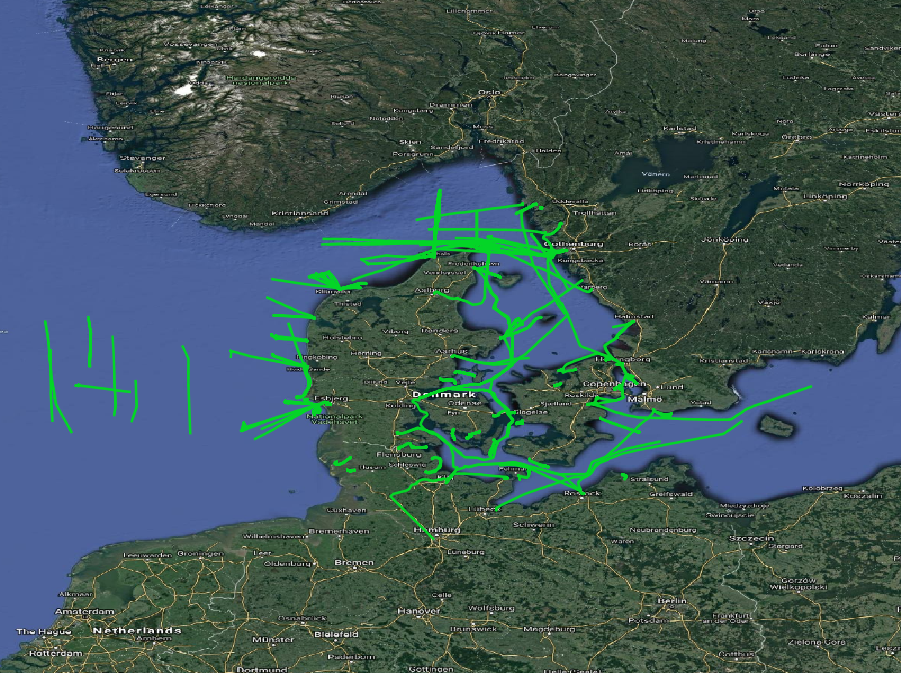
Surprisingly there are trips with zero length. These are clearly noise that can be deleted. Also there are very many short trips, that are less than 50 km long. On the other hand, there are few long trips that are more than 1,500 km long. Let's visualize these last two cases in Figure 1.3, “Visualizing trips with abnormal lengths”. They look like noise. Normally one should validate more, but to simplify this module, we consider them as noise, and delete them.

DELETE FROM Ships
WHERE length(Trip) = 0 OR length(Trip) >= 1500000;
-- Query returned successfully in 7 secs 304 msec.
				

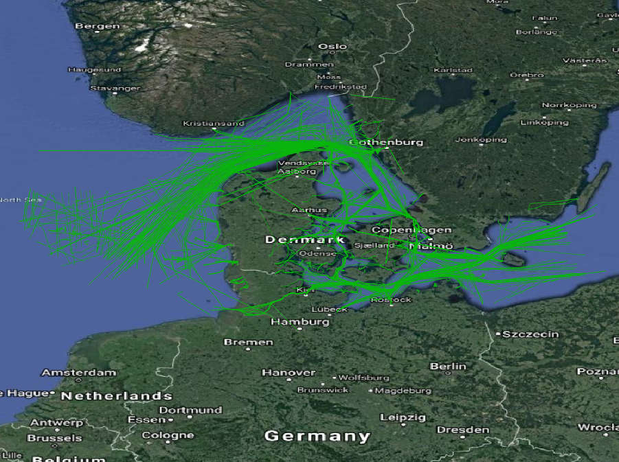
Now the Ships table looks like Figure 1.4, “Ship trajectories after filtering”.

Let's have a look at the speed of the ships. There are two speed values in the data; the speed calculated from the spatiotemporal trajectory speed(Trip), and the SOG attribute. Optimally, the two will be the same. A small variance would still be OK, because of sensor errors. Note that both are temporal floats. In the next query, we compare the averages of the two speed values for every ship:

SELECT ABS(twavg(SOG) * 1.852 - twavg(speed(Trip))* 3.6 ) SpeedDifference
FROM Ships
ORDER BY SpeedDifference DESC;
--Total query runtime: 8.2 secs
--990 rows retrieved.

SpeedDifference
NULL
NULL
NULL
NULL
NULL
107.861100067879
57.1590253627668
42.4207839833568
39.5819188407125
33.6182789410313
30.9078594633161
26.514042447366
22.1312646226031
20.5389022294181
19.8500569368283
19.4134688682774
18.180139457754
17.4859077178001
17.3155991287105
17.1739822139821
12.9571603234404
12.6195380496344
12.2714437568609
10.9619033557275
10.4164745930929
10.3306155308426
9.46457823214455
...
				

The twavg computes a time-weighted average of a temporal float. It basically computes the area under the curve, then divides it by the time duration of the temporal float. By doing so, the speed values that remain for longer durations affect the average more than those that remain for shorter durations. Note that SOG is in knot, and Speed(Trip) is in m/s. The query converts both to km/h.

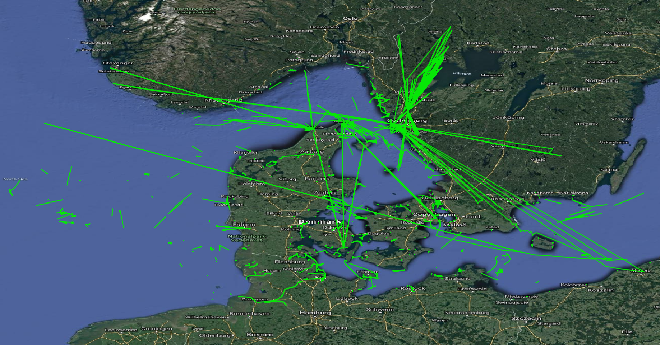
The query shows that 26 out of the 990 ship trajectories in the table have a difference of more than 10 km/h or NULL. These trajectories are shown in Figure 1.5, “Ship trajectories with big difference between speed(Trip) and SOG”. Again they look like noise, so we remove them.

Now we do a similar comparison between the calculated azimuth from the spatiotemporal trajectory, and the attribute COG:

SELECT ABS(twavg(COG) - twavg(azimuth(Trip)) * 180.0/pi() ) AzimuthDifference
FROM Ships
ORDER BY AzimuthDifference DESC;
--Total query runtime: 4.0 secs
--964 rows retrieved.

264.838740787458
220.958372832234
180.867071483688
178.774337481463
154.239639388087
139.633953692907
137.347542674865
128.239459879571
121.107566199195
119.843262642657
116.685117326047
116.010477588934
109.830338231363
106.94301191915
106.890186229337
106.55297972109
103.20192549283
102.585009756697
...
				

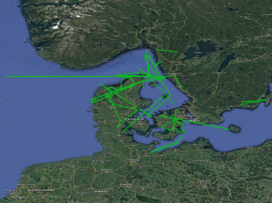
Here we see that the COG is not as accurate as the SOG attribute. More than 100 trajectories have an azimuth difference bigger than 45 degrees. Figure 1.6, “Ship trajectories with big difference between azimuth(Trip) and COG” visualizes them. Some of them look like noise, but some look fine. For simplicity, we keep them all.